

Rough contact from scratch in TriboSolver 3.1
Build a rough, normally loaded contact from scratch: define two steel bodies, generate a reproducible surface, calculate the pressure distribution, and export a report.
No bundled example or measured surface file is needed. We enter the settings tab by tab in the released Windows application. The screenshots, numerical outputs and report previews below come from the same tutorial run.
1. Simulation Type: choose Dry Contact
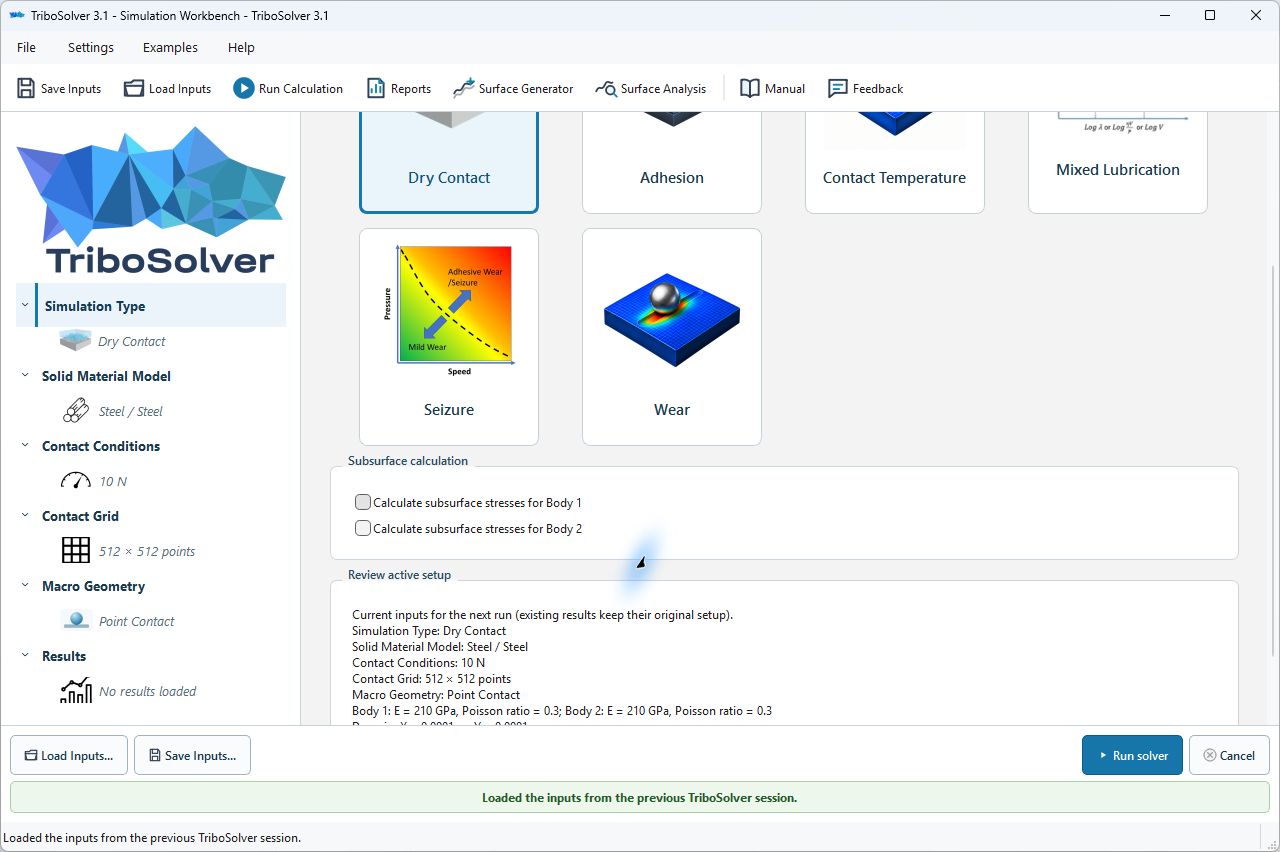
Open TriboSolver 3.1 with a valid licence. In Simulation Type, select Dry Contact. Scroll down and clear both Calculate subsurface stresses checkboxes. We want the surface pressure and deformation, without calculating stress volumes inside the bodies.
The application may restore your previous session. Do not assume the restored load, grid or geometry is correct: replace them with the values in the following steps. Do not select an item from the Examples menu.
2. Solid Material Model: define the two bodies
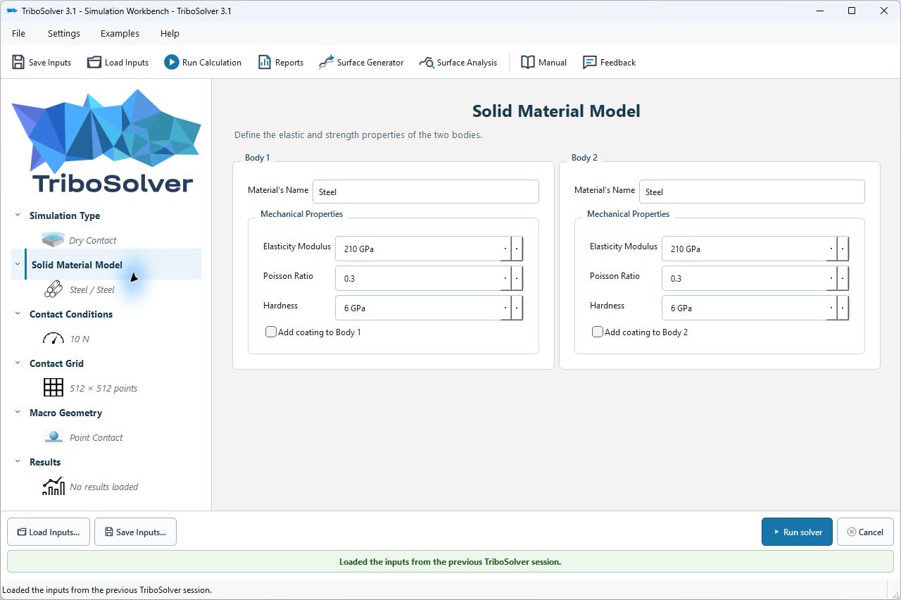
Open Solid Material Model. Select Steel for each body, then check the numerical values explicitly. Leave the coating options off.
| Parameter | Body 1 and Body 2 | Meaning in this case |
|---|---|---|
| Young's modulus, E | 210 GPa | Elastic stiffness: how strongly the body resists deformation. |
| Poisson's ratio, ν | 0.3 | Relates transverse to axial elastic deformation. |
| Hardness | 6 GPa | Material hardness supplied to the contact model. This run reports zero plastic surface deformation. |
| Coating | Off for both bodies | Use uncoated, homogeneous bodies. |
3. Contact Conditions: prescribe 1 N
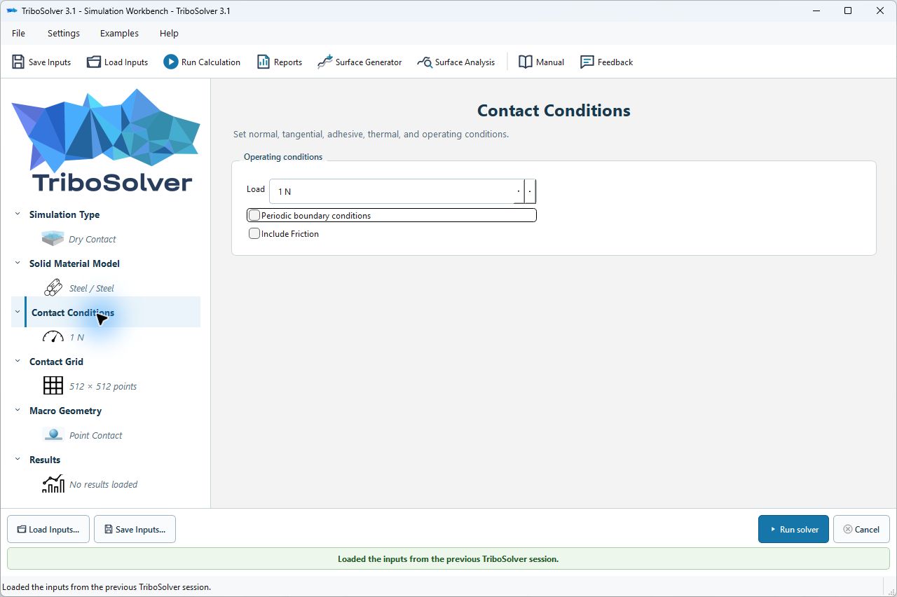
In Contact Conditions, set the normal load to 1 N. Leave friction and the periodic boundary option off. This is an isolated, normal-contact problem; sliding, tangential loading and repeated periodic contacts are not part of this tutorial.
4. Contact Grid: choose size and resolution
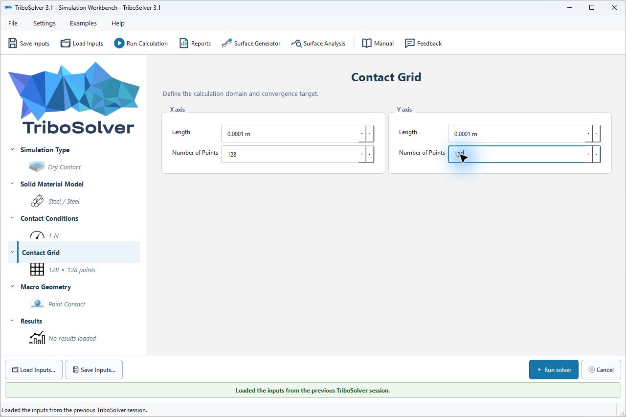
Set both domain lengths to 0.0001 m and both point counts to 128. The Contact Grid fields use metres: 0.0001 m equals 100 µm. Do not enter 100 in a field labelled m.
| Field | Enter | Physical interpretation |
|---|---|---|
| X length / Y length | 0.0001 m / 0.0001 m | A square 100 × 100 µm calculation domain. |
| X points / Y points | 128 / 128 | 16,384 surface-grid points; nominal spacing 0.78125 µm. |
Domain size and point count are different choices: one sets the physical area, the other its sampling. This modest grid makes a convenient introductory calculation. Engineering conclusions require a separate domain-size and mesh-refinement assessment.
5. Macro Geometry: create a point contact
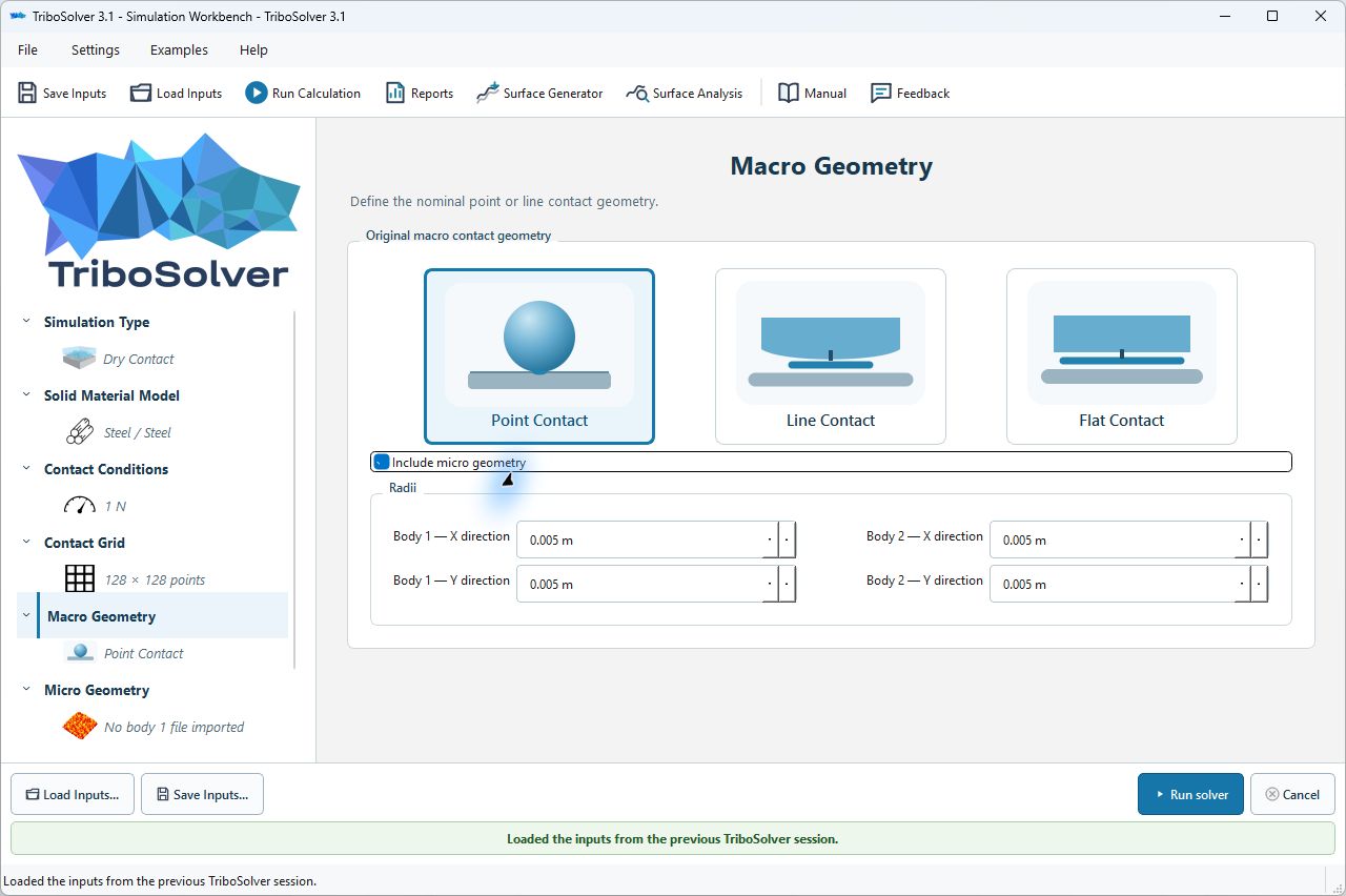
Select Point Contact. Enter 0.005 m in all four radius fields: Body 1 X, Body 1 Y, Body 2 X and Body 2 Y. These represent two equally curved convex bodies, not a sphere on a flat plane. Enable Include microgeometry to expose the roughness setup.
Combining two 5 mm convex radii gives an effective radius of 2.5 mm in each direction: 1/Reff = 1/R1 + 1/R2. The large-scale curvature defines the overall contact shape; the generated roughness perturbs it locally.
6. Micro Geometry: generate a reproducible rough surface
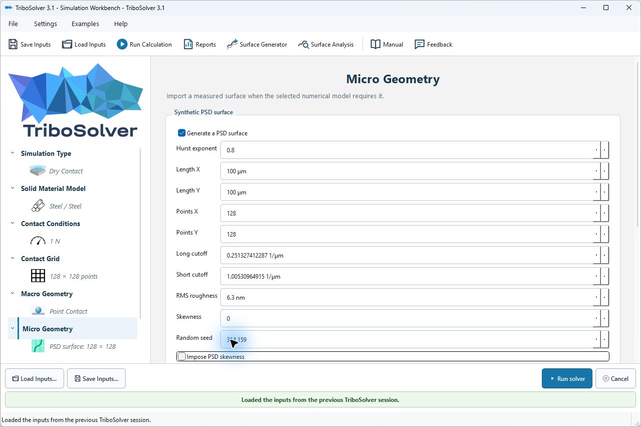
Open Micro Geometry and enable Generate a PSD surface. PSD means power spectral density: it describes how roughness is distributed over spatial frequencies. Enter the values below; do not import a surface file.
| Field | Enter in the UI | What it controls |
|---|---|---|
| Hurst exponent | 0.8 | The scaling of the synthetic roughness across spatial frequencies. |
| Length X / Length Y | 100 µm / 100 µm | Match the physical contact domain. |
| Points X / Points Y | 128 / 128 | Match the contact grid. |
| Long cutoff | 0.251327412287 1/µm | Low-wavenumber boundary of the generated spectrum; enter a reciprocal length, not a wavelength. |
| Short cutoff | 1.005309649149 1/µm | High-wavenumber boundary. The displayed last digits may round after entry. |
| RMS roughness | 6.3 nm | Root-mean-square variation of height about the mean. |
| Skewness | 0; Impose PSD skewness off | No imposed skewness constraint. The finite generated surface need not have exactly zero measured skewness. |
| Random seed | 314159 | Reproduces the same realization when the generator settings are unchanged. |
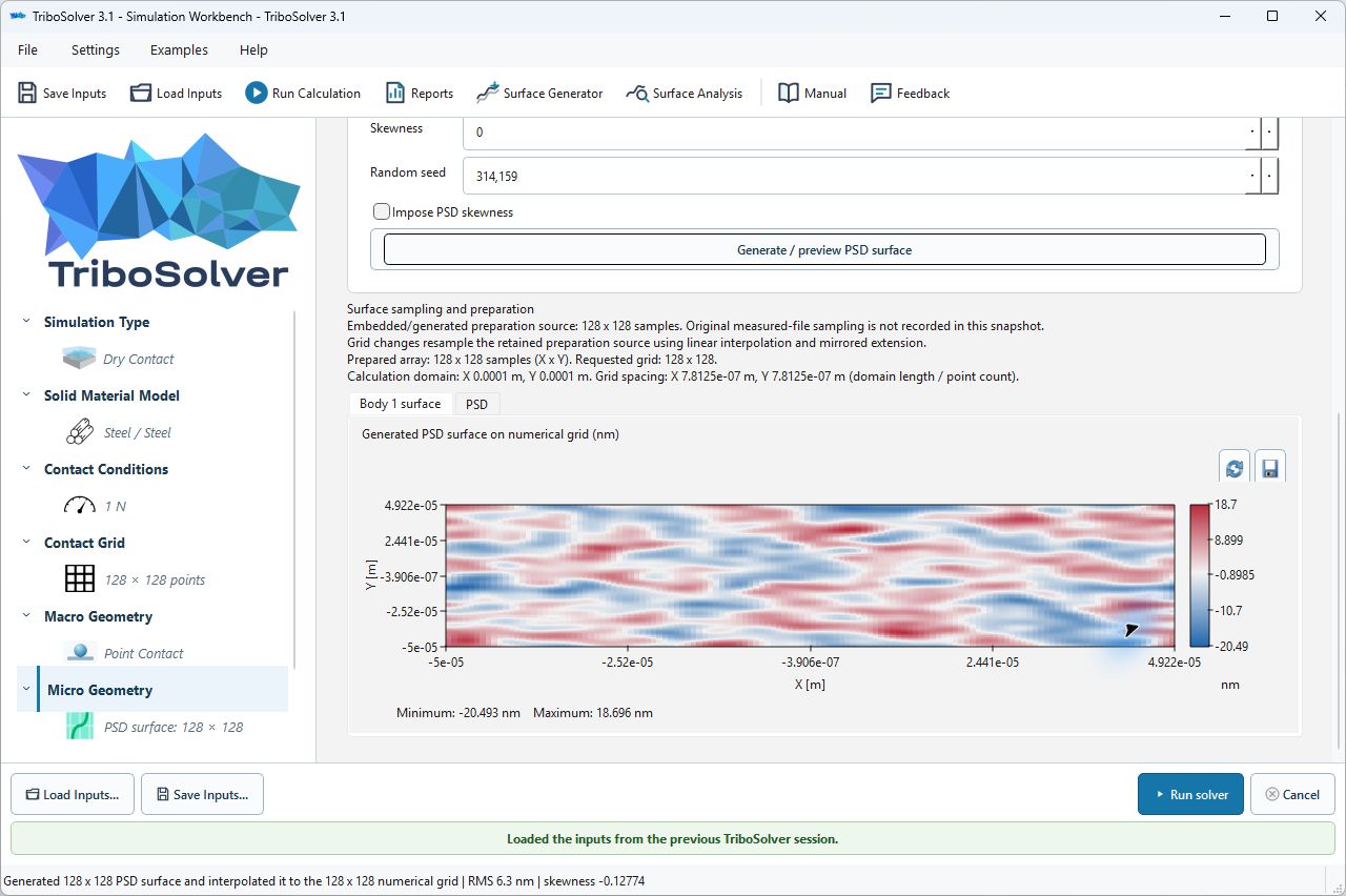
Click Generate / preview PSD surface. Inspect the Body 1 surface preview before running. For this seed, the generated surface has RMS 6.3 nm, measured skewness −0.12774 and heights from −20.493 to 18.696 nm. The map's X/Y axes are in metres; its colour scale is height in nanometres. Read the axes rather than interpreting the on-screen plot's stretched aspect ratio as the physical shape.
7. Save the setup and run the calculation
Review the sidebar: Dry Contact, Steel / Steel, 1 N, 128 × 128 points, Point Contact and the generated PSD surface. Use Save Inputs to keep a named setup, then click Run Calculation (or Run solver at the bottom).
This run used contact-equilibrium tolerance 10−6 and a maximum of 3,000 contact iterations. If you changed numerical settings in a previous session, check them before comparing. Wait for a convergence message; merely seeing a plotted result is not a convergence check.
8. Results: understand the pressure and contact area
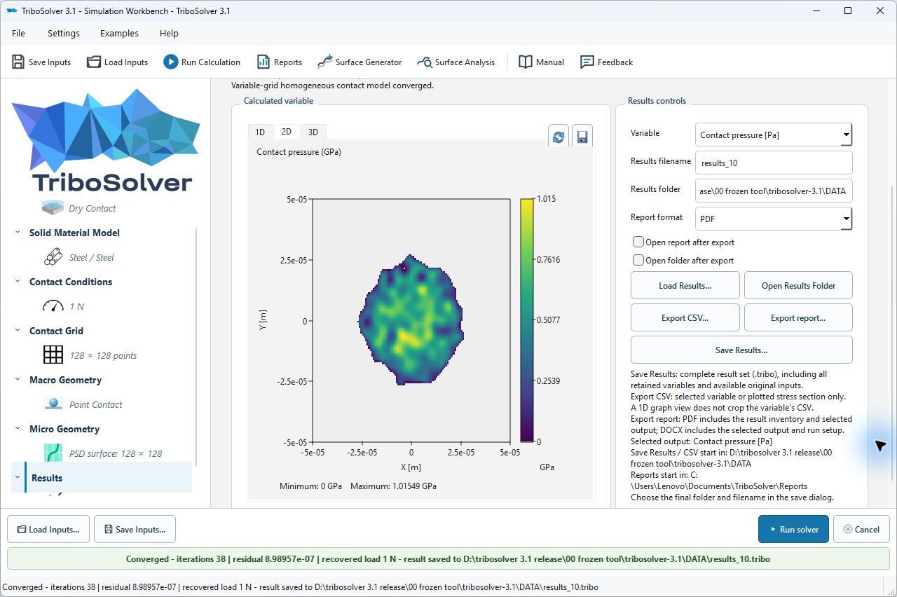
Open Results and select Contact pressure. The colour map shows the pressure at each point; the peaks are not uniform because the generated roughness redistributes the load.
| Output | This tutorial run | How to read it |
|---|---|---|
| Calculated contact load | 1.000000 N | Balances the prescribed normal load of 1 N. |
| Peak pressure | 1.01549 GPa | Largest value in the full pressure map. |
| Contact area | 2.011108 × 10⁻⁹ m² 2,011.11 µm² | Area in contact, approximately 20.11% of the full domain. |
| Average contact pressure | 0.497238 GPa | Load divided by the actual contact area, not the whole domain. |
| Nominal area / pressure | 10,000 µm² / 0.100000 GPa | The full domain area and load divided by that area. |
| Rigid body motion | 0.256771 µm | The calculated overall approach parameter, distinct from the roughness amplitude. |
| Iterations / final residual | 38 / 8.98957 × 10⁻⁷ | The residual is below the selected 10−6 tolerance. |
Why is the average below the peak? Load is shared over many contacting grid points. Some carry more pressure than others; a local maximum is therefore different from load divided by contact area. Likewise, averaging over the entire domain includes the non-contacting region and gives the lower nominal pressure.
Other outputs include elastic displacement, plastic surface deformation and a contact-area map. The plastic-deformation output is zero for this run. Inspect labels carefully: exported surface fields can include prepared contact geometry, so they should not be confused with the isolated generated roughness preview above.
9. Save results and export a report
Use Save Results to keep the calculated result set. This is separate from Save Inputs, which preserves the configuration. In the Results report controls, select PDF, click Export report and choose your output filename and folder.
The following are the first two pages of the report exported from this run: a summary with key outputs, followed by the pressure map and centre X cross-section. Click either image to read it at full size.
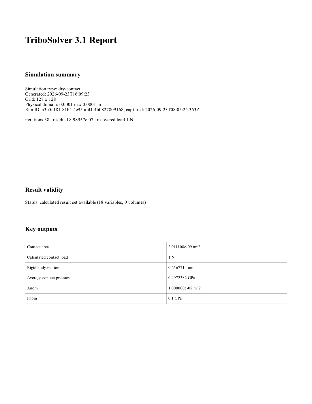
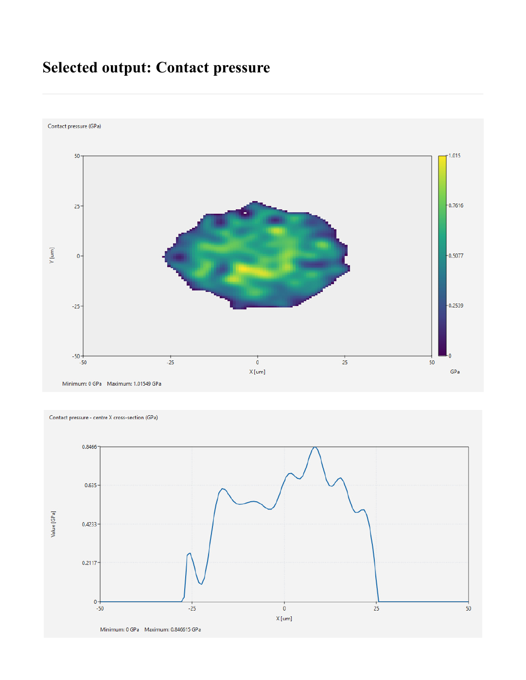
The centre-line curve peaks at about 0.846615 GPa, below the full-map maximum of 1.01549 GPa: the largest pressure lies away from that particular slice. The report's input appendix also retains settings for other model families; its simulation type, dry-contact, identifies the calculation performed here.
Watch the setup walkthrough
Follow the same setup in this faster, English-narrated screenshot walkthrough, lasting about 1 minute 52 seconds. Pause at any step to enter the values, or use the tables above for a detailed reference.
The written steps provide the settings and explanations used in the video. Screenshots and report previews are from the released TriboSolver 3.1 application.