

Build a smooth, elastic point-contact calculation in TriboSolver 3.1, one tab at a time. Then compare the pressure and contact area with the analytical Hertz solution for the same material pair, load and effective radius.
1. Select the simulation physics
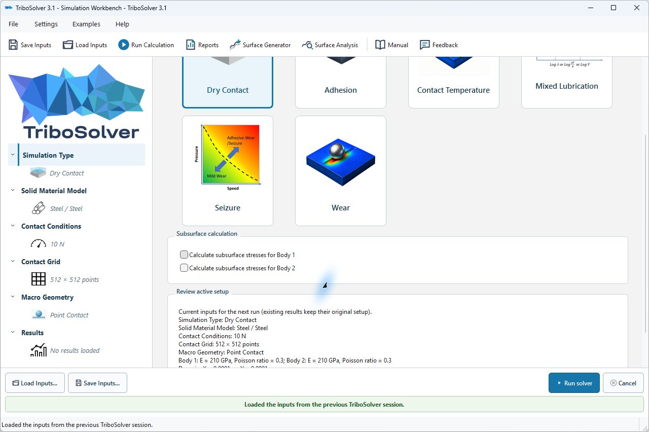
Open the released TriboSolver 3.1 application with your licence. In Simulation Type, select Dry Contact. Clear the subsurface-stress checkboxes for both bodies. Do not load an example: enter the following settings yourself, checking any values restored from your last session.
2. Define both steel bodies
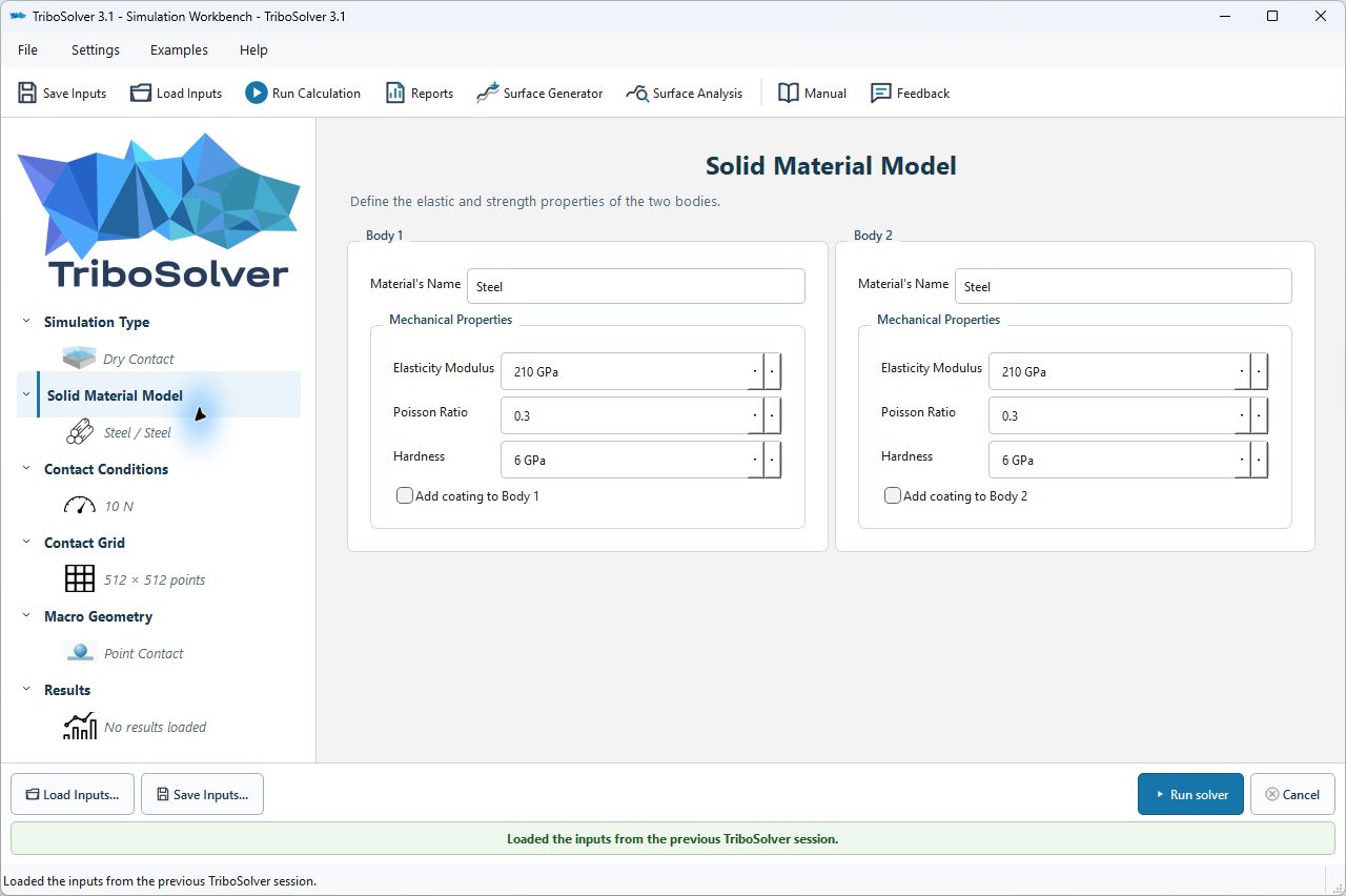
Open Solid Material Model and select Steel for Body 1 and Body 2. Set Young's modulus to 210 GPa, Poisson's ratio to 0.3 and hardness to 6 GPa for each body. Leave both coating options off.
Young's modulus controls elastic stiffness; Poisson's ratio relates transverse and axial deformation. Both bodies contribute to the effective stiffness. The supplied hardness is above the pressures in this case, and the result reports no plastic surface deformation.
3. Apply the normal force
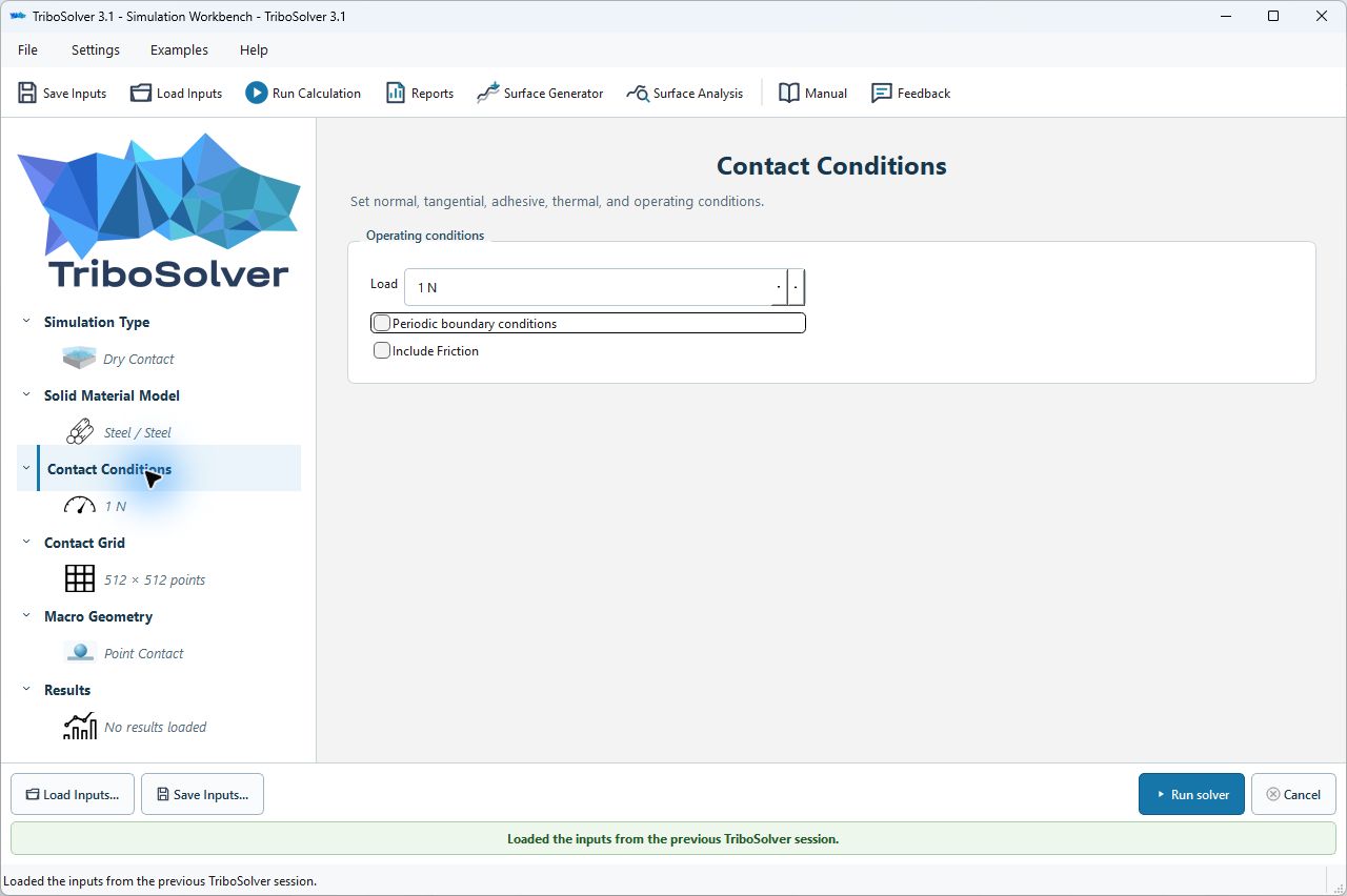
In Contact Conditions, enter 1 N. Disable friction and periodic boundaries. The analytical comparison below is for an isolated, normally loaded, smooth elastic contact; it does not represent sliding or an adhesive contact.
4. Set the domain and grid
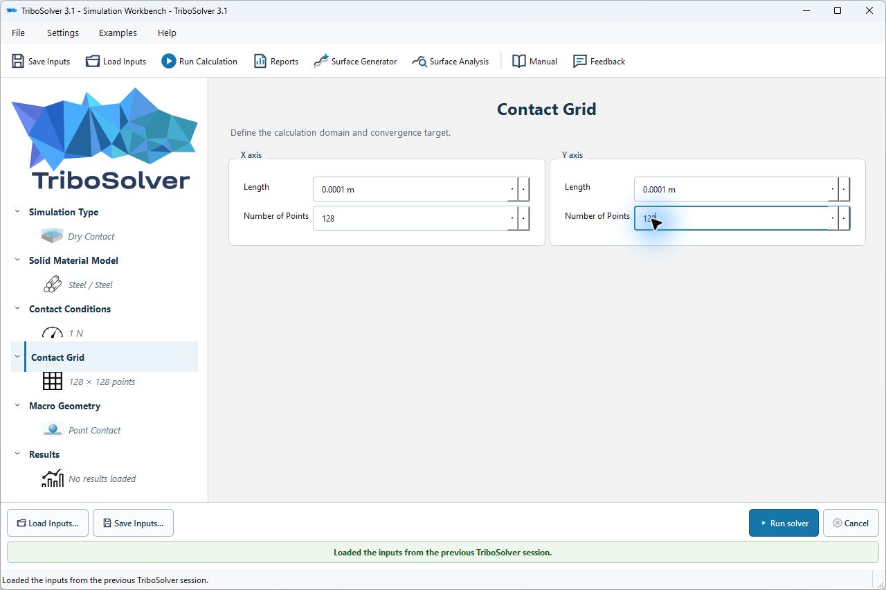
In Contact Grid, enter 0.0001 m for each domain length and 128 for both point counts. The physical domain is 100 µm wide in X and Y. Be careful with units: the fields use metres, so entering 100 would not mean 100 µm.
The anticipated Hertz contact radius is about 25.33 µm, so this domain extends beyond the contact in both directions. The 128 × 128 grid is the resolution used for the results below, not proof of mesh independence. Check domain size and grid refinement separately when developing an engineering case.
5. Create a smooth point contact
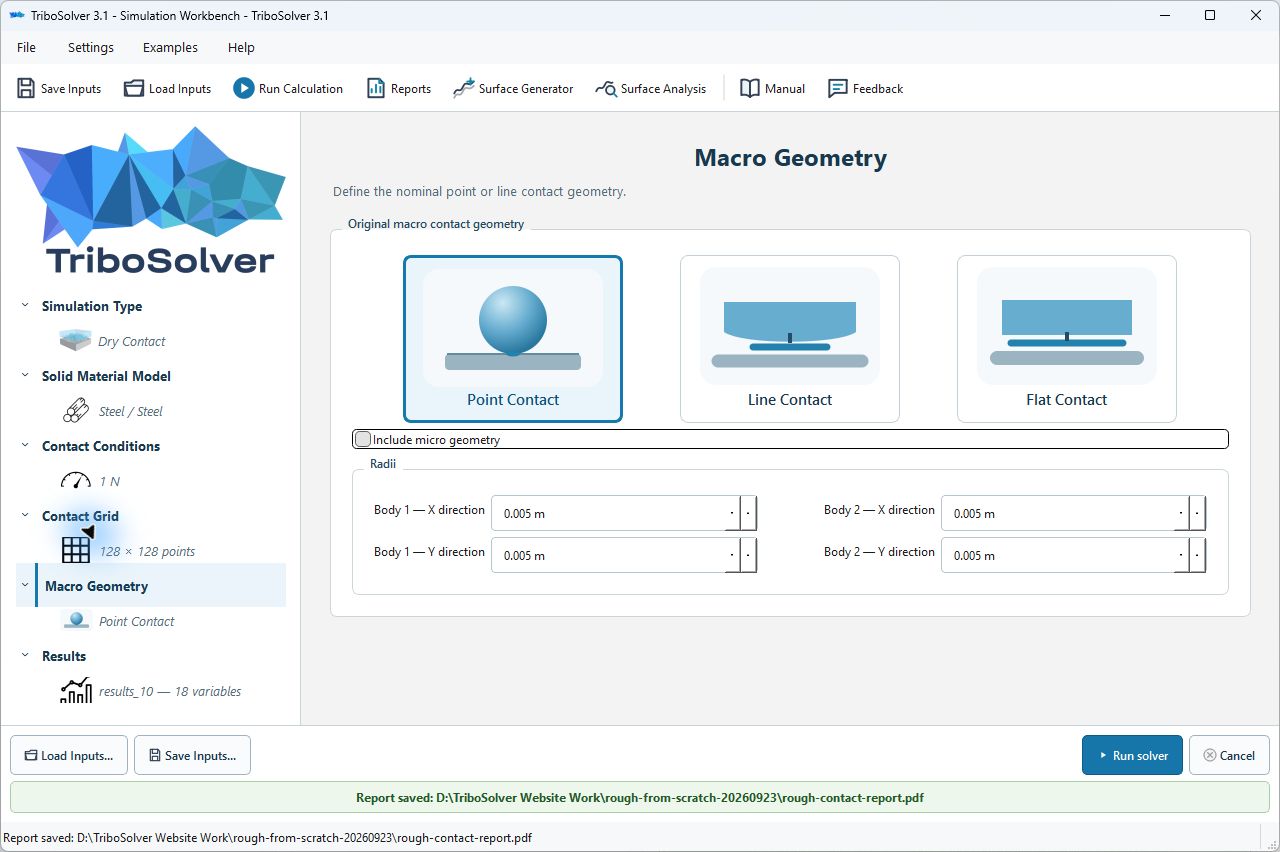
Open Macro Geometry and select Point Contact. Enter 0.005 m in all four radius fields: X and Y for Body 1, and X and Y for Body 2. Clear Include microgeometry. No surface import or PSD generation is required.
These are two convex curved bodies, not a sphere on a plane. Combining their radii gives 1/R = 1/R₁ + 1/R₂, so the effective radius R is 0.0025 m. Equal effective radii in X and Y give the circular Hertz special case.
6. Save inputs and calculate
Use Save Inputs to preserve your configuration. Choose a distinct results filename so an earlier run is not overwritten. Review the load, materials and grid, then press Run Calculation or Run solver.
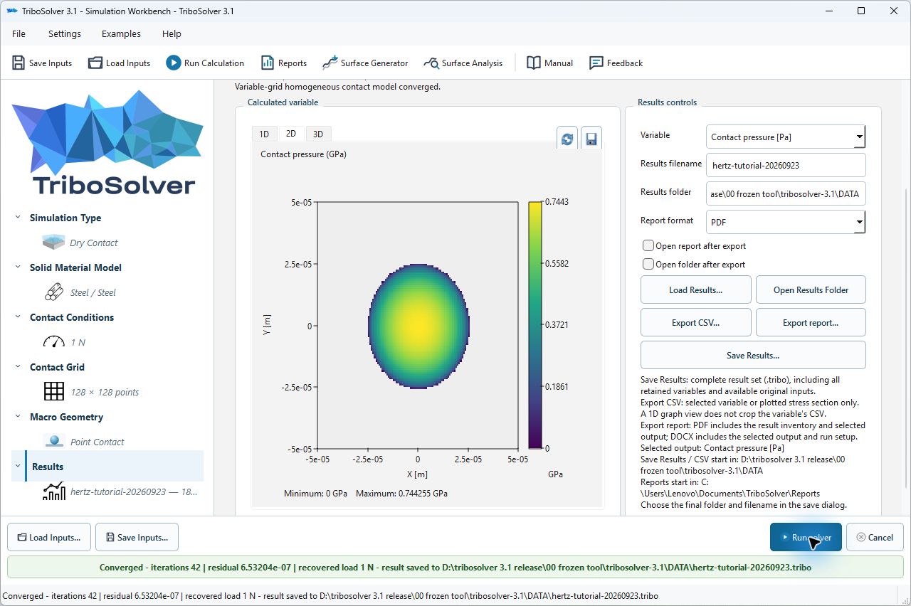
This calculation used a contact-equilibrium tolerance of 10−6 and a maximum of 3,000 contact iterations. It converged in 42 iterations, with residual 6.53204 × 10⁻⁷, and recovered the prescribed 1 N load. Open Results and select Contact pressure.
7. Compare the numerical result with Hertz theory
For this circular, smooth elastic contact, calculate the effective modulus from 1/E* = (1 − ν₁²)/E₁ + (1 − ν₂²)/E₂. Then a = (3FR/4E*)1/3, A = πa², p₀ = 3F/(2πa²), and approach δ = a²/R. These standard relationships are documented in the CompuTiX Hertz reference.
Here E* = 115.385 GPa and the analytical contact radius a = 25.3290 µm. The table compares the actual saved numerical outputs with reference values calculated from these inputs. Relative difference is (calculated − reference) / reference × 100%.
| Quantity | Calculated | Hertz reference | Relative difference |
|---|---|---|---|
| Peak pressure, GPa | 0.744254698 | 0.744227664 | +0.00363% |
| Contact area, µm² | 2,024.5361 | 2,015.5123 | +0.44772% |
| Approach, µm | 0.256611850 | 0.256622994 | −0.00434% |
| Recovered load, N | 1.000000 | 1.000000 prescribed | 0.00000% at shown precision |
The pressure is greatest near the centre and falls towards zero at the boundary. The calculated average contact pressure is 0.493940 GPa: load divided by the actual contact area. The nominal pressure is only 0.1 GPa, because it divides the same load by the entire 10,000 µm² domain.
The contact-area difference is larger than the peak-pressure difference. The numerical contact edge is resolved on a finite grid; a close peak match does not establish accuracy of every output. These comparisons describe this one tutorial run, not a general guarantee or a completed refinement study.
8. Save results and export the report
Use Save Results to retain the calculation. In Results, choose PDF and click Export report, then select a filename and folder. Save Inputs and Save Results serve different purposes: keep both when documenting a calculation.
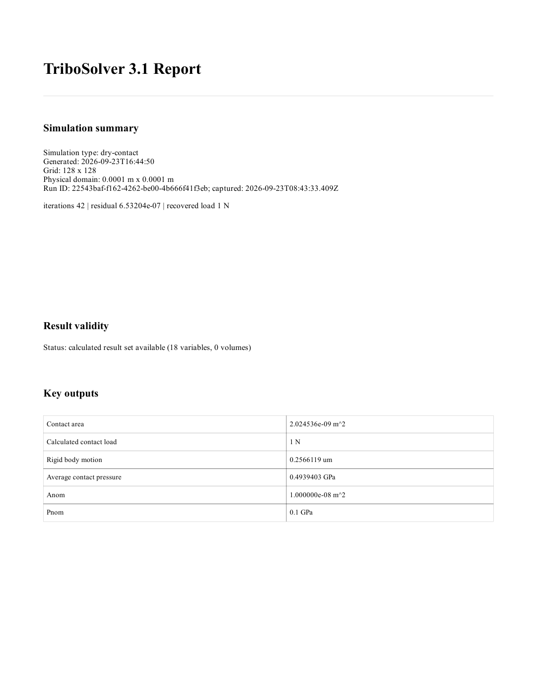
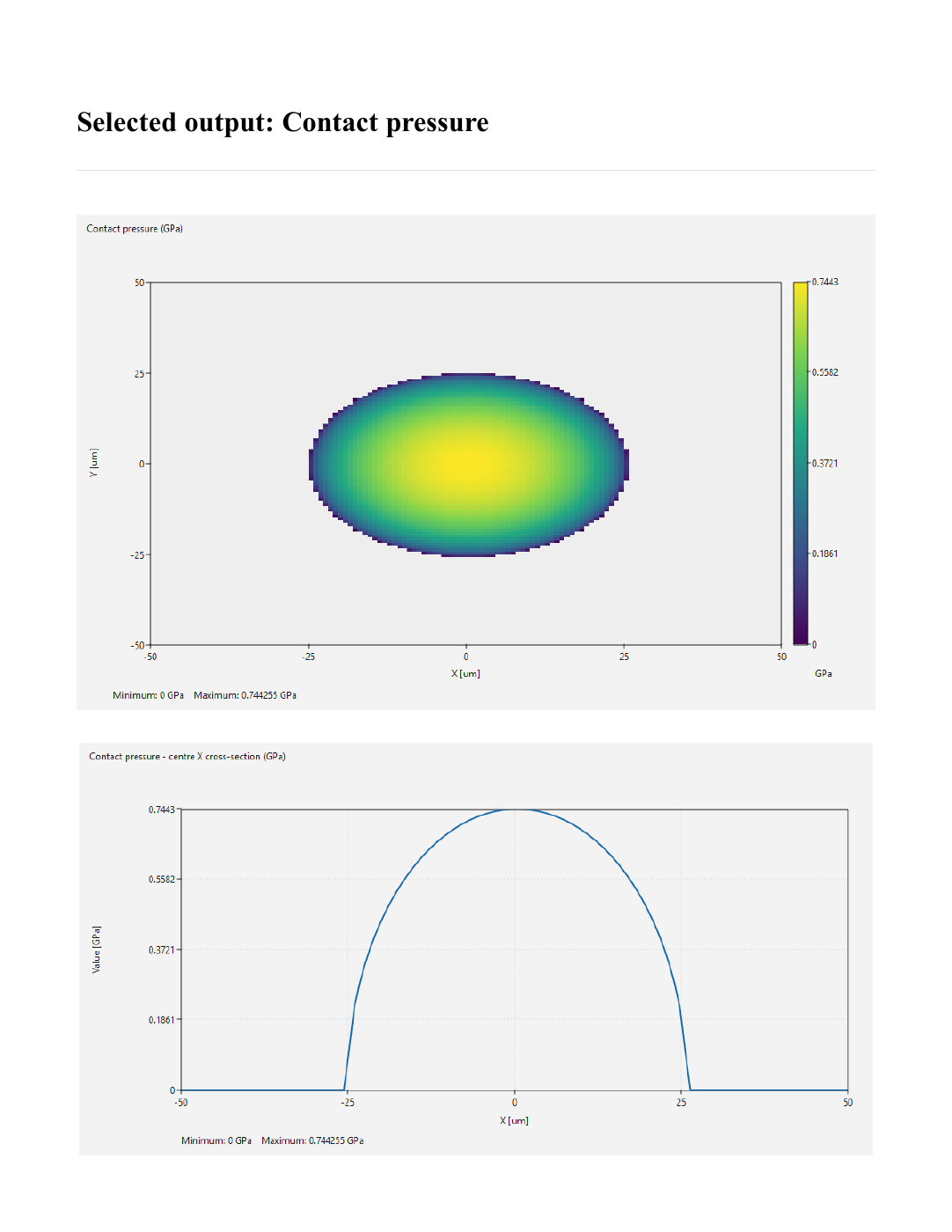
The first page summarizes the run and key outputs. The second shows the pressure map and centre X cross-section. Although the displayed map looks stretched, the coordinate ranges in X and Y are the same: this is a circular contact. Judge dimensions from the axes, not the plot's on-screen aspect ratio.
The report's input appendix may retain settings for other model families. The simulation type identifies which calculation was performed. This guide uses dry contact with microgeometry disabled.
Watch the narrated walkthrough
Follow the same manual setup in this short English-narrated screenshot walkthrough. Pause at any step to enter the values; the tables above provide the detailed settings and comparison.