

Rough Contact Problem Solution Using TriboSolver Online
Results from the current rough-contact example
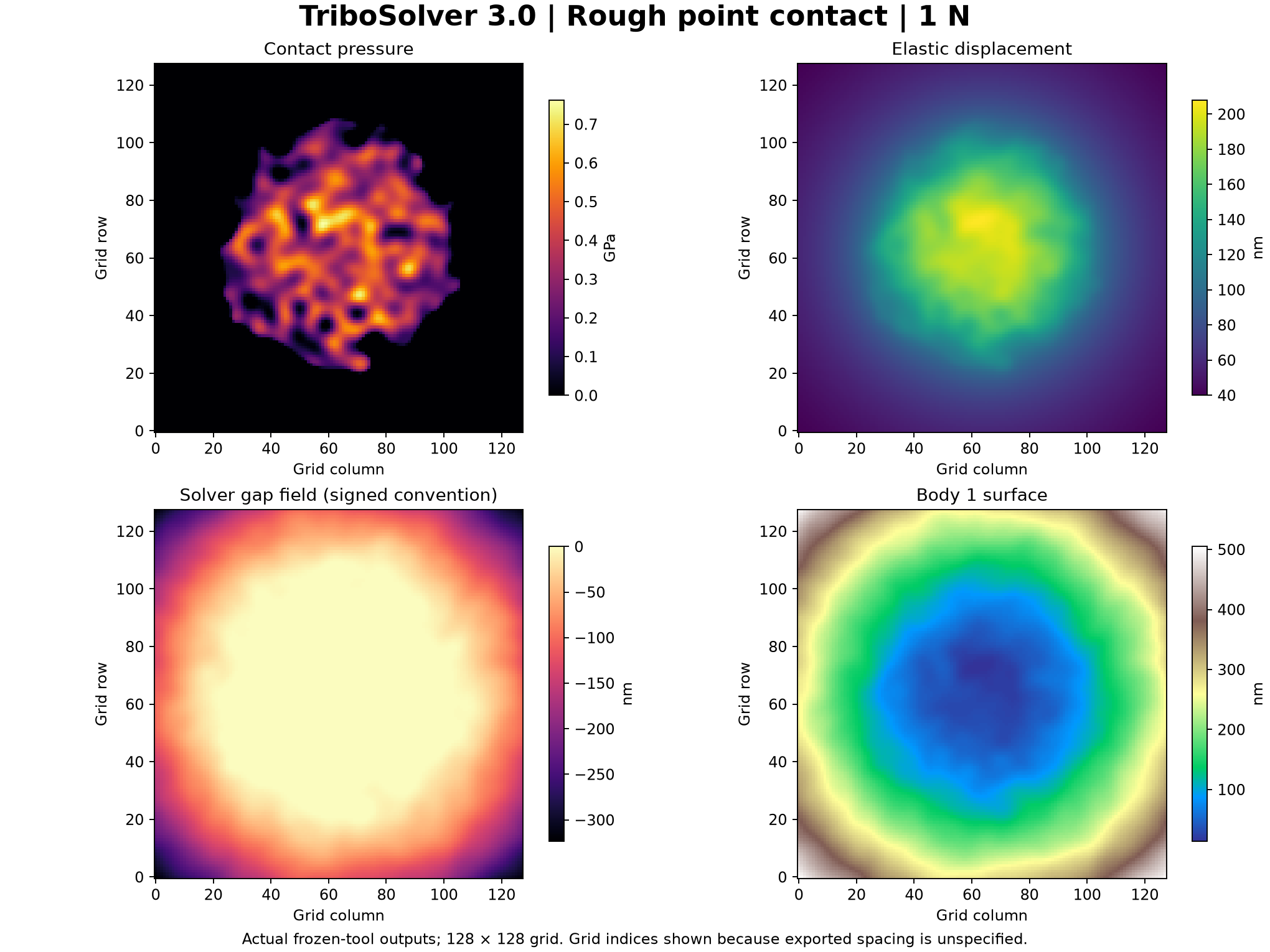
The run converged in 37 iterations with a reported residual of 9.11 × 10⁻⁷ and recovered load of 1 N. These are results from this example, not a general accuracy guarantee.
Reading the output variables
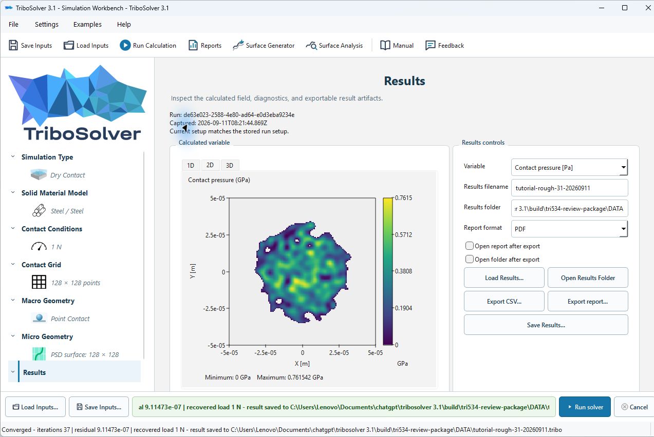
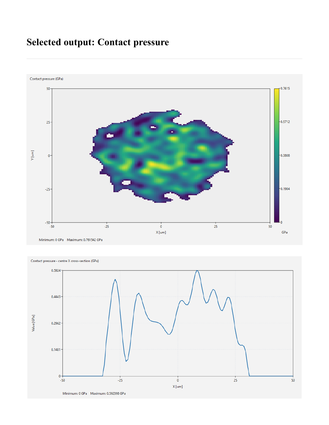
- PADIS — contact pressure: shown in GPa. Load is concentrated in separated patches; local peaks depend on surface resolution and mesh refinement.
- Elastic displacement: deformation field, converted to nm for this figure. The displacement extends beyond the regions carrying contact pressure.
- gap: the raw signed solver field, shown in nm. Negative values occur in the exported convention; do not interpret this plot as a non-negative film thickness or take its absolute value without checking the model definition.
- S1: the exported Body 1 surface field, shown in nm; this view includes the model geometry and is not a roughness-only microscope image.
- FC: recovered contact force in N; compare with the prescribed normal load.
- AREA: reported contact area in m². Distinguish it from Anom, the nominal area.
- Up: plastic displacement output; it is distinct from elastic displacement.
- Contact solver iterations / Final contact-equilibrium residual: convergence diagnostics, not experimental validation.
What the maps show
The pressure is heterogeneous rather than a smooth Hertz distribution, as expected for this generated rough surface. Inspect the pressure and surface maps together, then repeat at a finer grid before drawing conclusions about peak stress. Preserve the input file and generated-surface settings so comparisons use the same problem.
Follow the workflow in TriboSolver 3.1
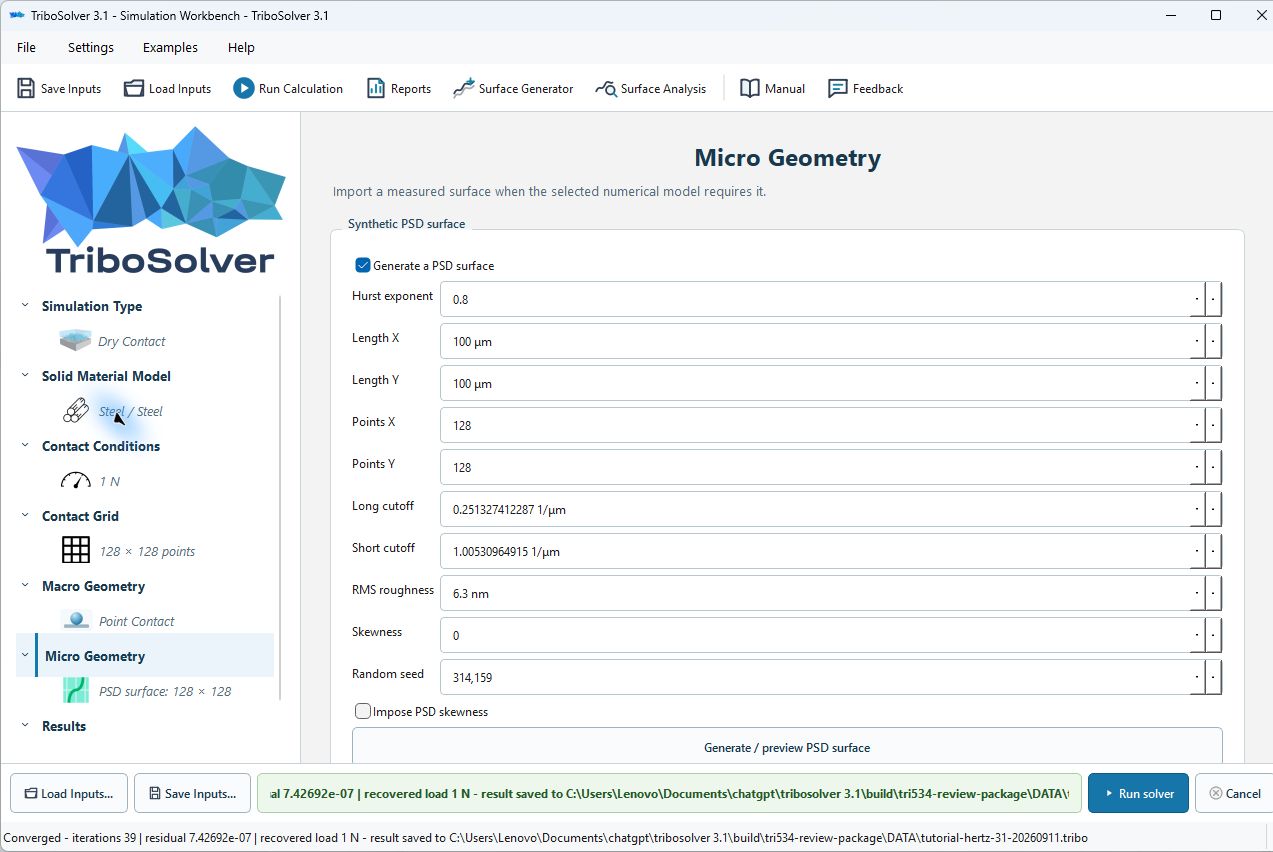
These are real captures from the 3.1 review application, using the tutorial inputs. They illustrate the interface and report layout; they do not replace the frozen 3.0 numerical comparison above or imply that 3.1 is the released download.
Setup and results screens
Open full-size image (new tab)
Open full-size image (new tab)
What the exported report looks like
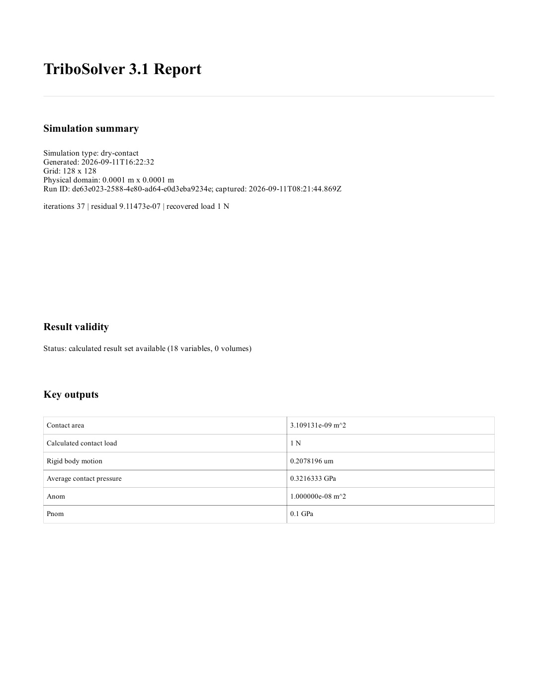
From Results, choose PDF and Export report. The following are the first two pages exported by the application for this case, not a redesigned report mock-up.
Open full-size image (new tab)
Open full-size image (new tab)
Read the report carefully: contact area is the calculated contacting area; Anom is the nominal domain area. Average contact pressure uses the contacting area, while Pnom uses the nominal area. Rigid body motion is the reported approach. The PDF uses µm (shown as um in some tables), metres squared and GPa as labelled. A centre-line maximum can be lower than the maximum over the whole map. Map panels are not drawn with equal X/Y display scales: use the coordinate values to judge dimensions, not the apparent aspect ratio. Retained settings for disabled models may appear later in the report; they do not mean those models were active.
Historical example and earlier-version video

Comments (2)
Leave a comment
You must be logged in to post a comment.
Begum Demirkurt
February 26, 2024I guess that the online simulator is not working at the moment, even though the simulation runs, there are no results…. I have already tried to reach you by sending several emails… I’m looking forward to your reply as soon as possible.
Aydar
February 29, 2024Thank you, Begum! Now the problem is solved!